


The Graph View
Introduction
VocBench, in addition to the Data Structure View (trees and
lists), provides a further way to explore data: the Graph View.
The Graph View comes in three perspectives:
- Data-oriented: it is a close representation of the RDF graph, with nodes representing resources and edges representing properties.
- Model-oriented: it is oriented to the relations that describe the ontology model, like the relations between the domain and range classes of a property.
- Class-diagram: it is oriented to describe relations among classes of an ontology.
Data-oriented graph
As stated in the introduction, this prospective is a close representation of the RDF graph. The nodes represent resources and the edges represent properties. Basically, each node-edge-node connection represents a subject-predicate-object statement.
A data-oriented graph can be accessed from three different points:
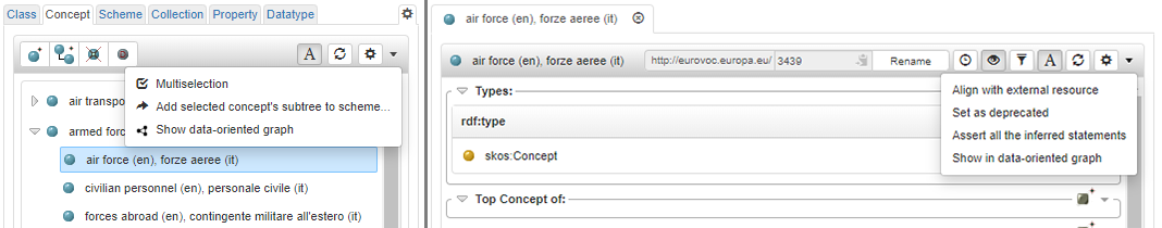
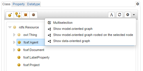
- The context menu of any tree or list panel (see figure below). It opens the Graph View rooted on the selected resource and expands it immediately. This menu entry is available only when a resource is selected.
- The context menu of a ResourceView (see figure below). It opens the Graph View rooted on the described resource and expands it immediately.
- In the SPARQL view, at the bottom of the results set of a graph-query by clicking on the button [
 ]. It opens the Graph View describing the statement returns by the query.
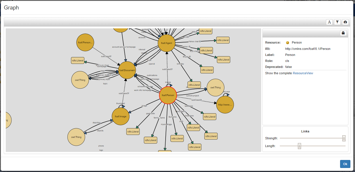
The Graph view is basically composed by a single panel splitted in two main sections: the left one which shows the graph and the right one containing a panel that shows a brief description of the selected node. At the bottom of the right panel there are also two sliders that allow to change the strength and the length of the links.
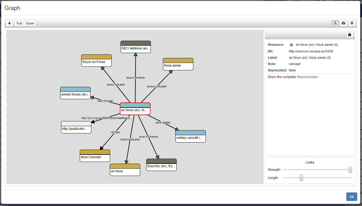
In the data-oriented graph, each node is represented by a rounded-corners rectangle with a top stripe. This stripe
gives an immediate idea of the nature of the resource described in the node. It could be seen as an alternative to
the resource icon used elsewhere, indeed, as shown by the previous figure, the selected node represents a concept
and its top stripe has a light-blue color, very similar to the concept icon.
The edges represent the predicates whose arrow indicates the direction of the relation: from the subject to the
object. As well as for the nodes, also the edges adopted a color code to explicit the nature of the predicate (as
much as possible more similar to the color of the icons), for example the object properties are rendered with a
blue arrow, the annotation properties with a yellow one, the datatype properties with a green one, and so on.
Every element of the graph, be it a node or an edge, when clicked is highlighted with a red border. Then the resource represented by the node is briefly described in the right panel from where it is possible to open the complete ResourceView. On the top on this panel, a lock button allows to lock/unlock the node position and so avoid that the node moves around the graph "pushed" by the graph forces. Every node can be expanded by double-clicking on it and collapsed in the same way.
On the left side of the panel heading are available the following actions:
- Add (the + button): allows to drag-in a new node choosable by exploring the same tree/list which the root resource belongs to (e.g. the concept tree if the graph is rooted on a concept)
- Expand sub-resources (the Sub button): expands the selected node by adding the resources related to it via hierarchical parent-child relations (e.g. if the node represents a concept, add its narrowers). This action is available only if a node is selected.
- Expand super-resources (the Super button): expands the selected node by adding the resources related to it via hierarchical child-parent relations (e.g. if the node represents a concept, adds its broaders). This action is available only if a node is selected.
On the right side there are three other buttons:
- Rendering (the A button): activates/deactivates the rendering of the nodes and edges labels.
- Export (the "camera" button): exports a snapshot of the graph in an .svg file. Note that the exported SVG shows the graph exactly how it is visible in the panel, namely if any graphic element is cut off from the gray area, it will be shown in the same way in the .svg file.
- Settings (the "gear" button): allows to edit the settings of the graph, in particular the filters on the visible elements.
Graph filters
With a growing amount of visual element (nodes and edges), the Graph View could be confused and it could reflect
in a decrease of performance, so, in the attempt to provide a better user experience, in the data-oriented Graph
View has been provided a filter mechanism.
There are available two kind of filter: a global filter, that is applied whenever a user expands a node, and a
local one, duly applied when the expansion of a node would produce too many nodes.
The "global" filters can be managed in the settings modal dialog.
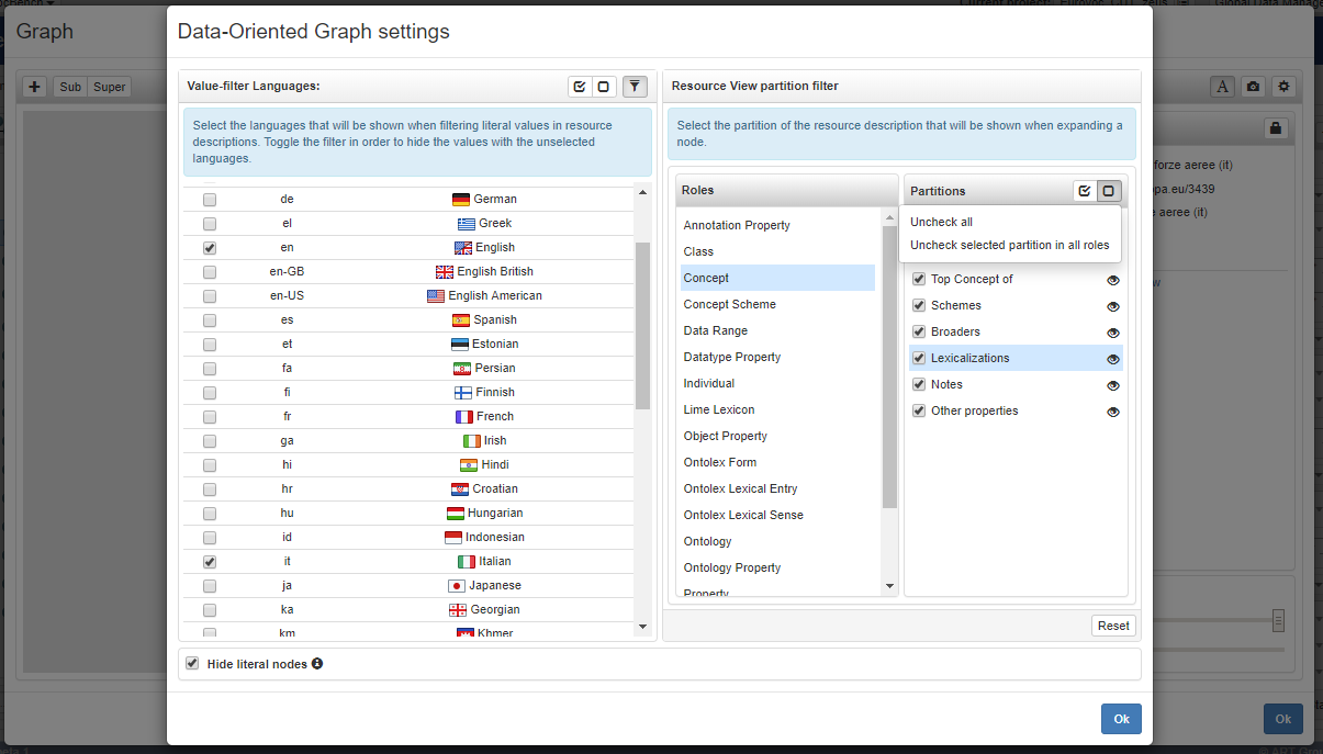
The panel Value-filter Languages, on the left side, allows to limit the literal nodes in the graph. Indeed,
from the languages list it is possible to enable/disable the visualization of literal nodes (or generally language
tagged resources) having the specified language, or even completely hide them all through the checkbox on the
bottom. Note that this filter is the same used in the ResourceView, so changes applied here will affect the
ResourceView and in the same way changes to the ResourceView filter will affect the graph.
The right panel allows to customize the expansion of the nodes according the role of the described resource. For
each role, it is possible to let expand or to cut off an entire partition (the partitions are the same used
in the ResourceView). For example, unchecking the Lexicalizations, all the relations that in the
ResourceView are handled by this partition (e.g. rdfs:label, skos:prefLabel, ...) will be excluded
from the graph.
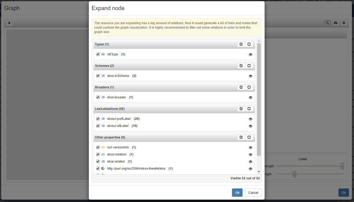
In some cases, the global filters might be not enough to limit the amount of element in the graph. If a resource has a large amount of relations, the expansion of the related node could produce a lot of links and nodes, so it will be proposed to filter the relations to be rendered. As shown in the figure below, a panel will let the user choose the partitions (or more specifically, the relations) to render.
Model-oriented graph
Unlike the previous graph type, in the Model-oriented graph the edges don't necessarily represent predicates but may represent more complex relations. Typical one, a class can be bound to another class via a property because that property has one class as its rdfs:domain and the other one as its rdfs:range.
The model-oriented graph can be accessed only from the context-menu of the class tree panel. It can be open by clicking on two different menu entries:
- Show model-oriented graph: allows the user to see the whole ontology under the model-oriented prospective. Note that in case of big ontologies, the visualization of the graph could be confusing and could be necessary to manually rearrange the nodes in a more ordered way.
- Show model-oriented graph rooted on the selected node: opens the Graph View rooted on the selected class and expands it immediately. This is particularly useful when the ontology in big and so allows to explore the graph incrementally. This menu entry is available only when a resource is selected.
When the graph is explored starting from a single class (graph opened through Show model-oriented graph rooted
on the selected node) the nodes of the graph can be expanded and collapsed in the same way seen for the
data-oriented graph. It is also possible to add a class, choosable browsing the class tree, to the graph.
On the contrary, when the graph is open through Show model-oriented graph, since it shows the whole
ontology, it is static, it cannot be explored and it is not possible to add further nodes.
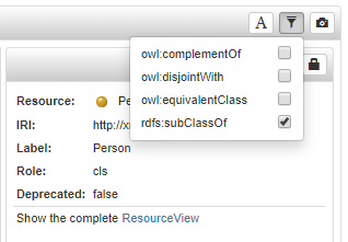
As well as for the data-oriented graph, through the buttons on the panel heading is possible to enable/disable the rendering and to export the graph as an .svg file. It is also available filter mechanism, simpler than the one in the data-oriented graph. As shown in the figure below, from the filter button can be enabled or disabled the visualization of four different class axioms.
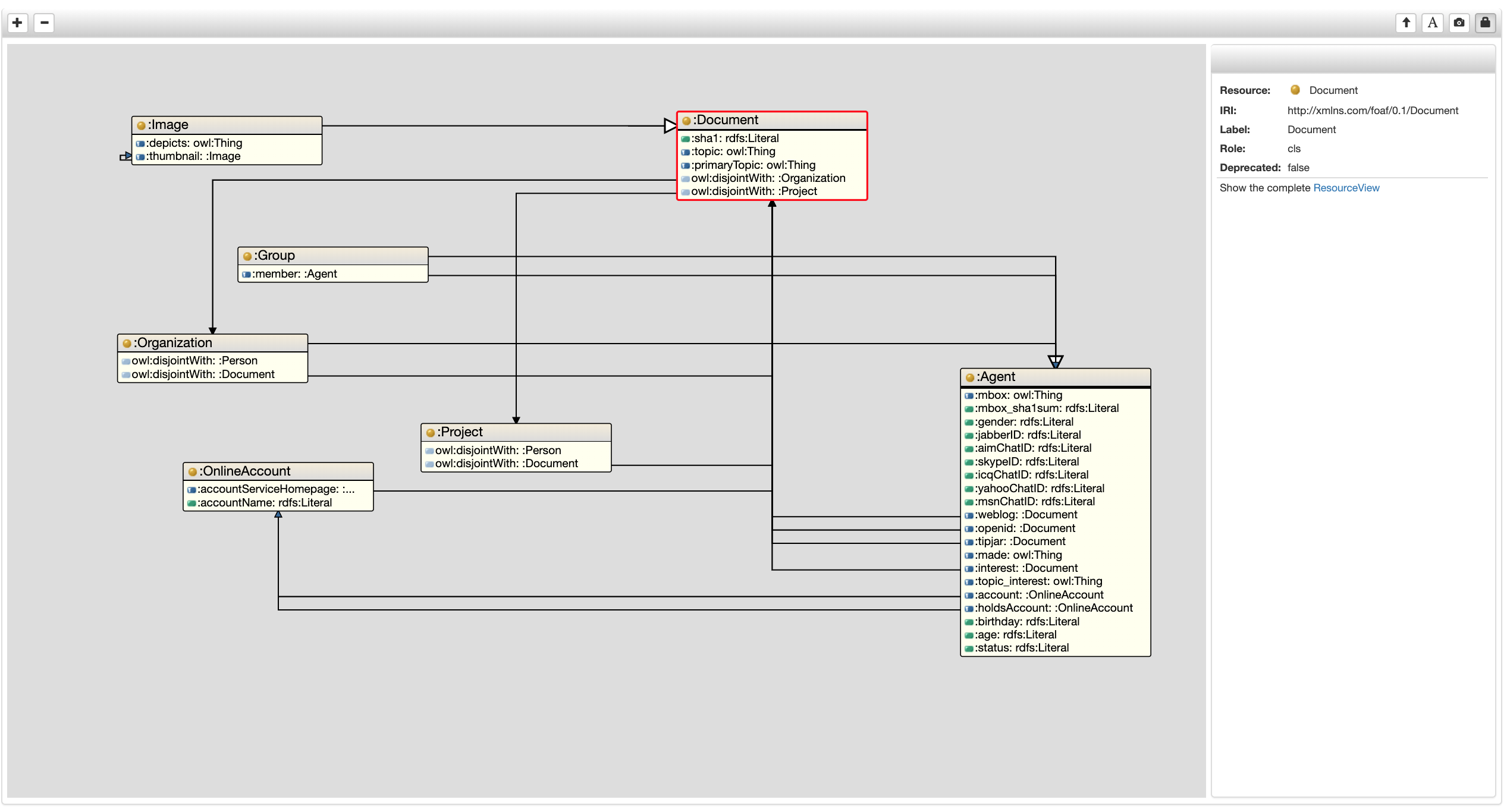
Class-diagram
In this graph, the nodes represent the classes of an ontology. Within classes, there are all properties have that class as their domain. For completeness to the domain has also been concatenated the range (separated by a small space). The links relate the domain of a specific property to its range. Below we will show first how to access the class-diagram and then the features implemented to manage it.
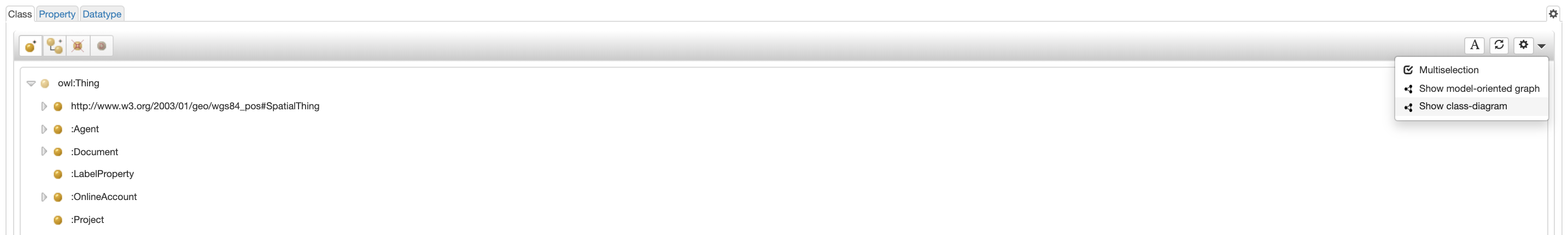
The class-diagram can be accessed only from the context-menu of the class tree panel. It can be open by clicking on "Show class-diagram" menu entry and allows the user to see the whole ontology under the class-diagram prospective.
As mentioned in the description of the previous graphs, also the class-diagram view is composed of a single panel split into two main sections: the left one which shows the graph and the right one containing a panel that shows a brief description of the selected links, properties or nodes. Initially, the graph will be displayed in dynamic mode, so the nodes and links, which are subject to forces, move independently until the equilibrium of forces is reached. Using the button [![]() ], which is located on the right side of the top panel, you can fix the nodes and links to place them in the position that makes the legibility of the graph clearer.
], which is located on the right side of the top panel, you can fix the nodes and links to place them in the position that makes the legibility of the graph clearer.
Another feature made available to the class-diagram is to be able to choose whether to display links with properties other than "subClassOf" (or not).
This possibility makes the graph even more readable in case there are too many links. This is possible through the button[![]() ].
].
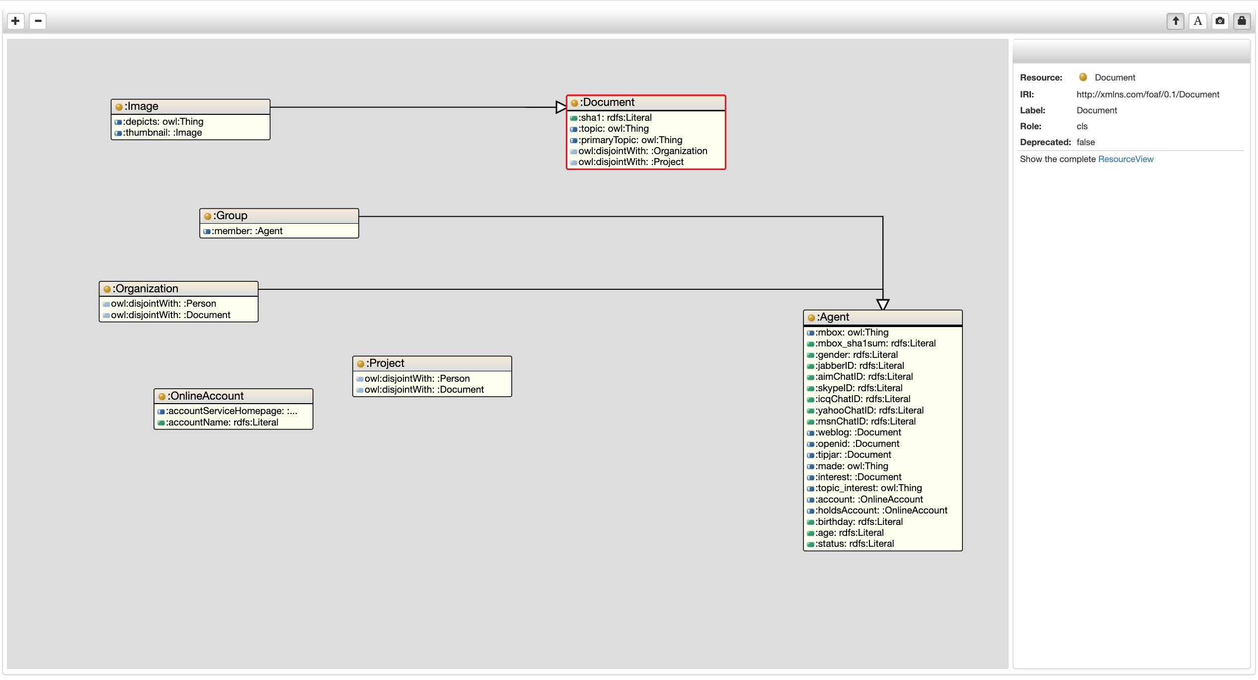
All the other functionalities in the panel remain the same as those previously described in the other paragraphs. The only difference is in the button[![]() ] that allows you to delete a class(with all its links) from the graph if you do not want to display it.
] that allows you to delete a class(with all its links) from the graph if you do not want to display it.